Automatic depth map generation, stereo matching, multi-view stereo, Structure from Motion (SfM), photogrammetry, 2d to 3d conversion, etc. Check the "3D Software" tab for my free 3d software. Turn photos into paintings like impasto oil paintings, cel shaded cartoons, or watercolors. Check the "Painting Software" tab for my image-based painting software. Problems running my software? Send me your input data and I will do it for you.
Bousseau et al. pioneered the process of watercolorizing a photograph in "Interactive watercolor rendering with temporal coherence and abstraction" by Adrien Bousseau, Matthew Kaplan, Joelle Tholot, Francois X. Sillion. The idea of darkening/lightening a color image given a grayscale texture image enables to simulate a bunch of watercolor effects including paper texture, turbulent flow, pigment dispersion, and edge darkening. There is another paper that I found quite useful in implementing my own version of Bousseau's watercolorizer, "Expressive Rendering with Watercolor" by Patrick J. Doran and John Hughes, as it discusses Bousseau's algorithm.
The first thing to do is to abstract the image in order to reduce the amount of details. Bousseau et al. uses Mean Shift to color segment the image followed by the application of morphological smoothing operators like dilation and erosion. Since I have already implemented software to abstract and stylize images (for cartoon rendering) in Non Photorealistic Rendering - Image Abstraction by Structure Adaptive Filtering, I simply use that to get the abstracted image. I think it works real good too.
Abstracted image.
Let's apply a watercolor paper texture to the abstracted image to simulate the grain of the watercolor paper.
Image after having applied a paper texture.
Let's apply a turbulent flow texture to the current image to simulate watercolor color variation due to how water moves and carries pigments. The turbulent flow texture comes from the sum of Perlin noise at various frequencies. It's mostly a low frequency coherent noise.
Image after having applied a turbulent flow texture.
Let's apply an edge darkening texture to the current image to simulate how pigments accumulate at the boundaries of washes. The edge darkening texture is obtained by computing the gradient magnitude of the original abstracted image.
Image after having applied an edge darkening texture.
Here's a video:
Bousseau et al. also use a grayscale texture to simulate pigment dispersion, the high frequency version of turbulent flow. It's supposed to be implemented as a sum of Gaussian noises. I don't really like that effect, so I simply did not implement it.
Clearly, this simulates the wet-on-dry watercolor technique, not the wet-on-wet technique. "Towards Photo Watercolorization with Artistic Similitude" by Wang et al. proposes a wet-on-wet effect which I will probably implement at some point.
Another stereo pair from the Peter Simcoe collection. As usual, first thing to do is to rectify the stereo pair using either er9b or er9c. This time I chose er9c.
Left image after rectification.
Right image after rectification.
Output from er9c:
Mean vertical disparity error = 0.362055
Min disp = -17 Max disp = 38
Min disp = -21 Max disp = 43
Time to generate the depth map. I am liking dmag6 more and more even though it is a memory hog and quite a bit slower than dmag5. For the min and max disparities, I will use min disp = -21 and max disp = 43.
Depth map obtained by dmag6.
Input to dmag6:
min disparity for image 1 = -21
max disparity for image 1 = 43
disparity map for image 1 = depthmap_l.png
disparity map for image 2 = depthmap_r.png
occluded pixel map for image 1 = occmap_l.png
occluded pixel map for image 2 = occmap_r.png
alpha = 0.9
truncation (color) = 30
truncation (gradient) = 10
truncation (discontinuity) = 10000
iteration number = 5
level number = 5
data cost weight = 0.5
disparity tolerance = 0
radius to smooth occlusions = 9
sigma_space = 9
sigma_color = 25.5
downsampling factor = 1
Let's improve the depth map by calling on our good friend dmag9b. For sure, dmag9b will sharpen the depth map at the object boundaries.
I don't like the depth map around the bags in the foreground and I really want the 2 thin straps near the bags to be included in the depth map. So, time to do some manual labor before calling on dmag4.
Sparse/scribbled depth map to be fed to dmag4. White areas are actually transparent.
If, when you start erasing with the eraser tool, you get white instead of the checkerboard pattern, it's because you need to add the alpha channel to the depth map.
Edge image to be fed to dmag4. White areas are actually transparent.
I use the paths tool to generate the edge image. It's easy as pie.
I have combined elements from two academic papers to create my own Stroke-Based Rendering (SBR) software. I used "Painterly Rendering with Curved Brush Strokes of Multiple Sizes" by Aaron Hertzmann for the general framework but I didn't particularly like his curved brush strokes. I prefer straight strokes with an oil paint texture. So, I turned to "An Algorithm For Automatic Painterly Rendering Based On Local Source Image Approximation" by Michio Shiraishi and Yasushi Yamaguchi to handle the brush strokes.
The following 2 images show the pseudo-code for the framework. They come straight from the Hertzmann paper.
The input is an RGB image (sourceImage) and a sequence of brush radii of decreasing size (R1 to Rn). The output is an RGB image (canvas) which is initialized to some middle gray color. For each brush radius, the source image is convolved by a Gaussain blur of variance f_sigma * Ri where Ri is the current brush radius. The parameter f_sigma is some constant factor that enables to increase or decrease the blurring. If f_sigma is set to a very small value, no blurring takes place. A layer of paint is then laid on the reference image (blurred source image) using the paintLayer function described below.
A grid is virtually constructed with a grid cell size equal to f_grid * R where f_grid is some constant factor and R is the current brush radius. Then, for each grid cell, he computes the average error within the grid cell, the error being defined as the difference in color between the current canvas color and the reference image color. If the average difference in color is greater than T (error_threshold), the pixel with the largest difference in color is chosen as the center of the brush stroke and that brush stroke is added to the list of brush strokes (the color for the brush stroke comes from the color of the pixel in the reference image). Once all the brush strokes have been created, they are randomized, and applied to the canvas.
As mentioned previously, I don't like curved brush strokes as I don't think it reflects particularly well what most fine art painters do. Straight brush strokes are in my opinion better and they are much easier to implement. Let's turn now our attention to the Shiraishi paper to make and paint the brush strokes.
The pixel with the largest error in the grid cell (its color is the brush stroke color) and the radius define a square window in the reference image. What Shiraishi does is create a grayscale difference image considering the brush stroke color as the reference color. He then uses image moments to define the equivalent rectangle of that square difference image. The center of the equivalent rectangle defines the brush stroke center. The angle theta between the longer edge of the equivalent rectangle and the x-axis defines the angle of the brush stroke. The width and length of the equivalent rectangle define the width and length of the brush stroke. This completely defines the brush stroke. Recall though that all brush strokes are made before they are applied onto the canvas.
To paint a given brush stroke, a rectangular grayscale texture image (where white means fully opaque and black means fully transparent) is scaled so that it matches the equivalent rectangle in terms of width and height, rotated by theta, translated so that its center matches the brush stroke center, and then painted onto the canvas using alpha blending. If you want to be real fancy and somehow simulate the impasto technique where thick layers of oil paint are applied, you may also use a rectangular grayscale bump map image alongside the texture image and a bump map alongside the canvas.
A few notes:
- I use a very small f_sigma so that the reference image never gets blurred. Because of that, the input image needs to be slightly blurred as high frequency artifacts could be a problem when evaluating the image moments.
- I always use f_grid = 1.0. That's why it's not a parameter.
- To render the bump mapping, I use Gimp as it has a very convenient bump map filter.
Here's a quick video:
At the moment, the software is sitting on my linux box but it is not available for download. If you like this type of painterly rendering, feel free to send me your photographs and it will be my pleasure to "paint" them for you.
This post describes all the parameters that impact the rendered image in "Image Abstraction by Structure Adaptive Filtering" by Jan Eric Kyprianidis and Jürgen Döllner. Note that this paper was seriously influenced by "Real-Time Video Abstraction" by Holger Winnemöller, Sven C. Olsen, and Bruce Gooch. If you are a bit confused by the title of the paper, "Image Abstraction by Structure Adaptive Filtering", you are not the only one. In layman terms, it's simply a cartoon filter.
Overview of the method (picture comes from the paper cited above).
I know a picture is worth a thousand words but I think that a picture and a thousand words are worth even more. So, let's try to explain what the method does in words. The first thing it does is to estimate the local orientation aka Edge Tangent Flow (ETF). Then, the input photograph is abstracted using a bilateral filter which happens to be separated (direction 1 is along the gradient and direction 2 is along the normal to the gradient). This bilateral filter that is used to iteratively abstract the original photograph is called "Separated Orientation Aligned Bilateral Filter" or "Separated OABF" or just OABF. Once the input photo is abstracted a bit, the edges are extracted using Difference of Gaussians (DoG) (The DoG is computed along the gradient and then smoothed using a one-dimensional bilateral filter along the flow curves of the ETF). This edge extraction method is called "Separated Flow-based Difference of Gaussians" or "Separated FDoG" or just FDoG. The input photo is abstracted some more using the same technique that was used prior to the edge detection. To give that cartoonish cel shading look, the image is then color quantized (using the luminance). The edges that were detected earlier are blended into the abstracted/quantized image to give the fully rendered image.
There are 2 parameters to control the number of iterations in "Separated OABF":
- n_e. That's the number of iterations before edges are detected. Kyprianidis uses n_e = 1 while Winnemöller uses n_e = 1 or 2.
- n_a. That's the total number of iterations (before and after edges are detected).
Parameters used:
- sigma_d. That's the variance of the spatial Gaussian function that's part of the bilateral filter. Both Kyprianidis and Winnemöller use sigma_d = 3.0.
- sigma_r. That's the variance of the color Gaussian function that's part of the bilateral filter. Both Kyprianidis and Winnemöller use sigma_r = 4.25.
For this step, the number of iterations used is the number of iterations before the edges are detected, that is, n_e.
Parameters used for the DoG filter that is applied in the gradient direction:
- sigma_e. That's the variance of the spatial Gaussian. The variance of the other spatial Gaussian is set to 1.6*sigma_e so that DoG approximates LoG (Laplacian of Gaussians). Larger values of sigma_e produce edges that are thicker. Smaller values produce edges that are thinner. Kyprianidis uses sigma_e = 1.0. Don't know about Winnemöller.
- tau. That's the sensitivity of edge detection. For smaller values, tau detects less noise but important edges may be missed. Kyprianidis uses tau = 0.99 while Winnemöller uses tau = 0.98.
Parameters used to smooth the edges in the direction of the flow curves:
- sigma_m. That's the variance of the Gaussian used to smooth the edges. The larger sigma_m is, the more smooth the edges will be. Kyprianidis uses sigma_m = 3.0. Don't know about Winnemöller.
Parameters used to threshold the edges:
- phi_e. Controls the sharpness of the edge output. Kyprianidis uses phi_e = 2.0 while Winnemöller uses phi_e between 0.75 and 5.0.
There is another parameter that can be used:
- n. That's the number of iterations of "Separated FDoG". Kyprianidis uses n = 1 most of the times. Don't know about Winnemöller.
In my humble opinion, the most important parameter when detecting the edges is sigma_e.
Step 4: Separated Orientation-aligned Bilateral Filter (2nd pass after the edges have been detected)
Parameters used:
- sigma_d. Same as before.
- sigma_r. Same as before.
For this step, the number of iterations used is the number of iterations that remain, that is, n_a-n_e.
Parameters used:
- phi_q. Controls the softness of the quantization. Winnemöller uses phi_q = 3.0 to 14.0.
- quant_levels. That's the number of levels used to quantize the luminance. Winnemöller uses quant_levels = 8 to 10.
At the moment, the software is sitting on my linux box but it is not available for download. If you like this cartoon rendering, feel free to send me your photographs and it will be my pleasure to cartoonify them for you.
This is called pseudo-quantization instead of quantization because it is based solely upon the luminance channel (of the CIE-Lab color space). The goal here is to simulate cel shading aka toon shading (just like it is done in cartoons). Of course, you'd better be not too picky otherwise you are going to be quite disappointed by the results. The main issue is how to handle the discontinuities between the quantized values: you don't want big color jumps especially in areas where the luminance gradient is small. If the quantized values are not smoothed in any way, then you have in your hands a hard quantization. If some efforts are made to smooth the transitions, it is soft quantization we are talking about.
A pioneer in this technique is Holger Winnemöller. So, let's take a look at "Real-Time Video Abstraction" and see how he handles quantization.
Quantization formula used by Winnemöller.
Quantized values for the luminance using a very small phi_q, a relatively small phi_q, and a relatively large phi_q.
Note that if phi_q is set to 0, the quantized values are q0, q1, q2, etc. As phi_q increases though, the quantized values change to q0+delta_q/2, q1+delta_q/2, q2+delta_q/2, etc. Winnemöller suggests using between 8 to 10 bins and a phi_q between 3.0 and 14.0. The transitions between quantized values are much smoother when phi_q is smaller (good!) but the (horizontal) steps are much shorter (not so good!).
Let's see the results of Winnemöller soft quantization on a real image ...
Image we want to color quantize.
Image quantized using 8 bins and phi_q = 3.0.
Image quantized using 8 bins and phi_q = 14.0.
Yeah, there's definitely quantization happening but not sure you are gonna be able to see the difference between the quantized images. Let's zoom in the upper right!
Image quantized using 8 bins and phi_q = 3.0 (zoomed in the upper right).
Image quantized using 8 bins and phi_q = 14.0 (zoomed in the upper right).
Clearly, the quantized image with phi_q = 3.0 has a smoother transition between flat areas of color than the quantized image with phi_q = 14.0. Kinda looks like the quantized image with phi_q = 3.0 is an anti-aliased version of the quantized image with phi_q = 14.0.
In the paper, Winnemöller is not satisfied with a uniform phi_q. Clearly, phi_q should be a function of the luminance gradient. Indeed, you kinda want phi_q to be relatively small when the luminance gradient is small and you want phi_q to be relatively large when the luminance gradient is large. All you have to do is compute the magnitude of the luminance gradient, clamp it on either end (min and max), and linearly interpolate phi_q between phi_q_min = 3.0 (corresponds to the min luminance gradient magnitude) and phi_q_max = 14.0 (corresponds to the max luminance gradient magnitude).
One can use the Difference of Gaussians (DoG) to extract edges from an intensity image. As you know, the Gaussian filter is a low-pass filter, meaning that it removes high frequency artifacts in an image (e.g. noise). When you take the Gaussian of an image and you subtract a larger sigma Gaussian from it, you essentially have a band-pass filter that rejects high frequency as well as low frequency intensities. That's perfect to detect edges! It should be noted that the edges we want when stylizing images are not necessarily the same edges one might want in other Computer Vision field. Indeed, we want relatively thick well-defined edges, not skinny edges like those you usually get with the Canny edge detector, for example.
To get started with computing the edge image, a one-dimensional DoG filter is applied along the gradient direction for every pixel in the input image (in CIE-Lab color space). It is customary to choose the variance of the 2nd Gaussian filter to be 1.6 times the variance of the 1st Gaussian. This is done so that the Difference of Gaussians (DoG) approximates the Laplacian of Gaussians (LoG).
Difference of Gaussians (DoG) filter applied in the gradient direction.
Now, in order to have nice flowing edges that would not be out of place in a Sunday morning paper funnies section, you need to smooth the edges along ... well, the edges. The problem is that it is those very nice flowing edges that we are trying to define. A chicken and egg problem, no doubt. Kang et al. in "Flow-based Image Abstraction" are the first ones to come up with a solution. They use the Edge Tangent Flow (ETF) vector field to smooth the edges. What you do is take the edge image coming from the DoG filter and convolve it along the flow curves of the ETF using a bilateral filter. It is very similar to the convolution used to visualize the ETF in Line Integral Convolution (LIC). For more info about ETF and LIC, check Non Photorealistic Rendering - Edge Tangent Flow (ETF).
We are not quite done yet as thresholding is applied to the edge image so that the grayscale values are (pretty much) either 0 (black) or 1 (white). A smooth step function function is used to control how sharp the edges are going to be.
Thresholding via smoothed step function.
Input rgb image.
Edge image obtained with Separated Flow-based Difference of Gaussians (Separated FDoG).
Bilateral filtering is a staple in the Computer Vision diet. It is used a lot to smooth images while preserving edges. The problem is that it is, in its naive implementation at least, quite slow especially if it needs to be iterated. As you probably know, the bilateral filter is a mix of two Gaussian filters, one that considers the spatial distance between the pixel under consideration and the neighboring pixel (in the convolution window) as the argument to the Gaussian function and one that considers the color distance. In contrast, the Gaussian filter is quite fast because it is separable, that is, you can apply a one-dimensional Gaussian filter along the horizontal and then apply another one-dimensional Gaussian filter along the vertical instead of applying a true two-dimensional Gaussian filter.
So, the bilateral filter is not separable. What can we do about that? Well, you can still separate the bilateral filter if you want to but it won't be the same. For some applications, it doesn't really matter if the implementation of the bilateral filter is not exact. So, you can separate the two-dimensional bilateral filter by applying a one-dimensional bilateral filter along the horizontal and then a one-dimensional bilateral filter along the vertical. If you have an Edge Tangent Flow (ETF) vector field handy, you can separate the bilateral filter by applying the one-dimensional bilateral filter along the gradient direction and the tangent direction alternatively. Recall that the gradient direction is perpendicular to the tangent direction and goes across the edge. This separation along the gradient and tangent is referred to as "Separated Orientation-Aligned Bilateral Filter" (Separated OABF) in "Image Abstraction by Structure Adaptive Filtering" by Jan Eric Kyprianidis and Jürgen Döllner. It is supposed to behave better at preserving shape boundaries than the non-oriented version (See "Flow-Based Image Abstraction"by Henry Kang et al.)
Before showing some examples of Separated OABF, it is probably a good idea to give the formula for the bilateral filter. You control the way the bilateral filter behaves by the variance "sigma_d" of the spatial Gaussian function and the variance "sigma_r" of the color (aka tonal or range) Gaussian function. The larger sigma_d, the larger the influence of far away (in the spatial sense) sampling points. The larger sigma_r, the less edge-preserving the filter is going to be.
The bilateral filter weights and formula.
Input rgb image (640x422).
Output from the "Separated Orientation-Aligned Bilateral Filter" (Separated OABF) using sigma_d = 16 and sigma_r = 16.
Given an input rgb image, given a pixel of that input rgb image, the eigenvectors of the so-called "structure tensor" (aka "2nd moment tensor") define the directions of extreme (minimum and maximum) rate of change (intensity rate of change). The eigenvector associated with the smallest eigenvalue defines the direction of minimum rate of change. The eigenvector associated with the largest eigenvalue defines the direction of maximum rate of change. If there is an edge at a given pixel, it is the eigenvector associated with the smallest eigenvalue that gives the direction of the edge. Indeed, if you go along the edge, the rate of change (in intensity) is minimum. So, for each pixel of the image, if you consider the eigenvector associated with the smallest eigenvalue, you have got yourself a vector field which is referred to as the Edge Tangent Flow (ETF) vector field. The name Edge Tangent Flow (ETF) comes from "Flow-Based Image Abstraction" by Henry Kang, Seungyong Lee, and Charles K. Chui. To get good results, the structure tensor should be smoothed a little using the usual Gaussian filter.
To visualize an Edge Tangent Flow (ETF) vector field, you can use Line Integral Convolution (LIC). What you do is start with a noise image where each pixel is given a random grayscale value. Then, for each pixel of the noise image, you follow the flow/stream line that passes through the pixel going forward and backward so that the pixel is in the middle of the flow/stream line under consideration. You convolve (with a one-dimensional bilateral filter) the values along that stream line and assign the resulting average value to the pixel. In the output grayscale image, the actual grayscale values have no meaning, that is, whiter does not mean a stronger edge.
Input rgb image.
Edge Tangent Flow (ETF) visualized by Line Integral Convolution (LIC).
With a good imagination, one can kinda see a Vincent Van Gogh or Edvard Munch style in the LIC visualization of an ETF. ETFs are used quite a bit in Non-Photorealistic Rendering (NPR), in particular, in Stroke-Based Rendering (SBR) or Painterly Rendering as they provide a simple way to orient brush strokes. ETFs are also used in image abstraction and stylization.
The original mpo file comes from Peter Simcoe at Design-Design. It was taken with a Fuji W3. The original dimensions are 3477x2016 pixels but I reduced the width to 1200 pixels mostly for my own convenience.
Left image (1200 pixels wide).
Right image (1200 pixels wide).
It is always a good idea to rectify the stereo pair before attempting to create depth maps. I use er9b (or er9c if er9b is too aggressive) to do so mainly because it also outputs the min and max disparities, which are usually needed by the automatic depth map generators. You can use StereoPhoto Makers to align but you will have to use df2 to manually get the min and max disparities.
Left image after rectification by er9b.
Right image after rectification by er9b.
Output from er9b (there's a whole lot more verbose from er9b but that's the important bit):
Mean vertical disparity error = 0.367249
Min disp = -21 Max disp = 16
Min disp = -23 Max disp = 15
Don't worry about the white areas in the left and right images as they will be cropped out after the depth map is obtained. They result from the camera rotations needed to align the stereo pair.
I am gonna use dmag6 to get the depth map using the min and max disparities coming from er9b. I could have used dmag5 with very similar results. We are only gonna consider the left depth map (associated with the left image) even though dmag6 outputs the left and right depth maps.
Input to dmag6:
min disparity for image 1 = -23
max disparity for image 1 = 16
disparity map for image 1 = depthmap_l.png
disparity map for image 2 = depthmap_r.png
occluded pixel map for image 1 = occmap_l.png
occluded pixel map for image 2 = occmap_r.png
alpha = 0.9
truncation (color) = 30
truncation (gradient) = 10
truncation (discontinuity) = 10000
iteration number = 5
level number = 5
data cost weight = 0.5
disparity tolerance = 0
radius to smooth occlusions = 9
sigma_space = 9
sigma_color = 25.5
downsampling factor = 1
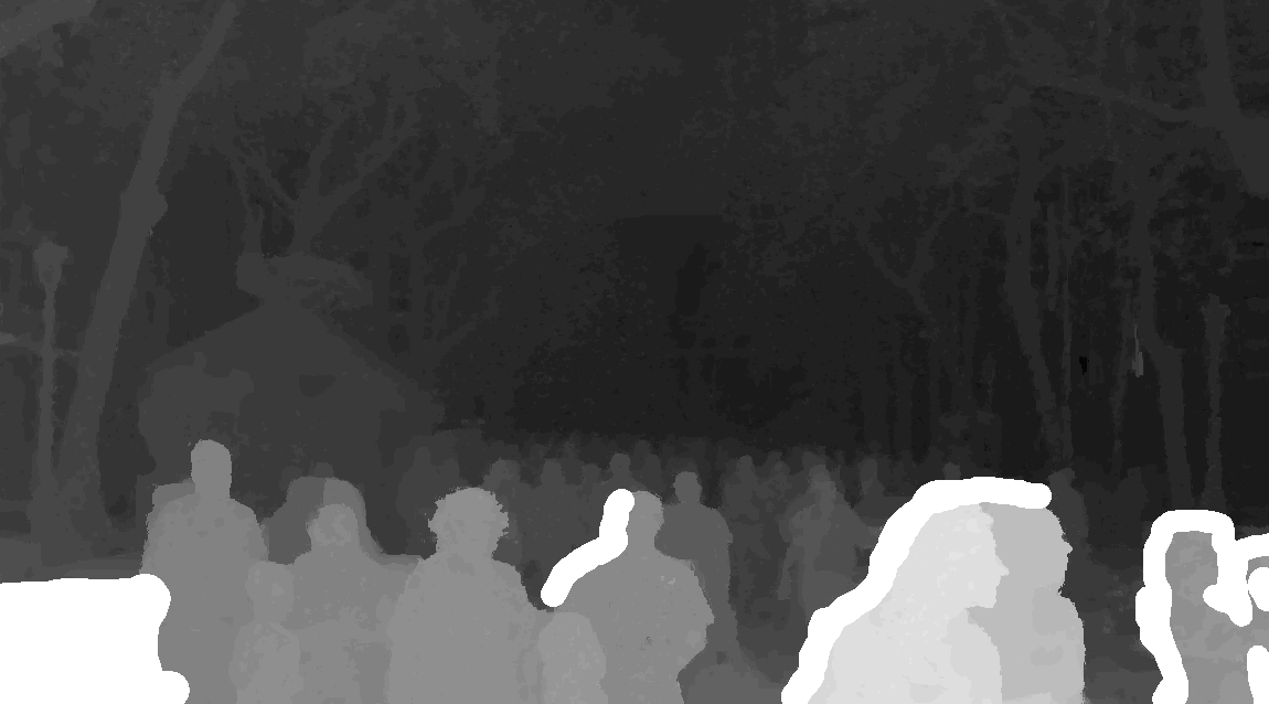
Depth map obtained by dmag6.
As promised, let's get rid of the artifacts coming from the rectification process by cropping the depth map and the reference image (left image).
Depth map obtained by dmag6 after cropping.
Reference image (left image) after cropping.
There are some areas in the foreground where the depth map is not that great. I am gonna use dmag4 to semi-automatically improve those areas. The input to dmag4 is the reference image which we obviously already have (that's the left image after cropping), the sparse/scribbled depth map, and the edge image.
To get the sparse/scribble depth map, you simply start with the cropped depth map and use the eraser tool (with anti-aliasing off, that is, hard edge on) to remove the areas you don't like, revealing the checkerboard pattern underneath. Of course, it's not the usual sparse/scribble depth map dmag4 usually takes for 2d to 3d conversion but it works just the same.
Input to dmag4 (sparse/scribbled depth map). The pure white areas are the areas that I erased. In gimp, they are transparent (checkerboard pattern) but blogger shows them as white.
To get the edge image, you simply trace the object boundaries in the areas that you erased in the sparse/scribbled depth map using the paths tool. The methodology in gimp is quite simple: create a path with the paths tool and then stroke it with anti-aliasing checked off and choosing a width of 1 pixel. Here, I use red for the color but you can use whatever color you want.
Input to dmag4 (edge image). What is shown as white in blogger is actually fully transparent (checkerboard pattern) in gimp.
As you can see, dmag4 fills the areas that were erased without spilling over the segmentation in the edge image. Because an edge image is used, beta needs to be relatively low (10 is a good value).
Wiggle 3d gif created by wigglemaker.
Any questions? Feel free to email me using the email address in the "About Me" box.