Stereo Matching - Variational Methods

Variational methods are global methods in the sense that they are trying to minimize a global energy function made up of two terms, "data" and "smoothness" (also referred to as "prior"). They are called variational methods because the energy is minimized using a mathematical tool called "Calculus of Variations" and in particular the Euler-Lagrange equations. Variational methods have become quite popular in the solution of the optical flow problem, where one estimates the displacement field between two images. Optical flow and stereo correspondence are not that much different. Optical flow is two-dimensional (the displacement field is two-dimensional, that is, objects may move in the x and y directions) while stereo correspondence usually assumes the displacement field is one-dimensional (the disparity is along the x-axis after rectification).

When an energy over a domain needs to be minimized and is of a certain form (see below), the solution of the so-called Euler-Lagrange equations minimizes the energy. Lucky for us, the energies used in optical flow and stereo correspondence are usually of the right type.


Euler-Lagrange equations in 2 dimensions.

If I1 is the left image and I2 the right image, if (u,v) represents the displacement, we want: 1) I2(x+u,y+v) to be equal to I1(x,y) for each pixel (x,y) and 2) a smooth displacement field. The following shows how to obtain the Euler-Lagrange equations for the optical flow/stereo matching problem with the assumption that the displacements are small (enables the linearization of the intensity in image 2 and makes the whole thing a lot much easier to solve):


Optical flow/stereo matching Euler-Lagrange equations.

At each pixel (x,y), you therefore have 2 equations. The derivatives can be evaluated using finite differences. Each system of 2 equations can be solved quite easily with an iterative scheme.

The process of minimizing the data energy term (for small displacements) can be easily visualized if we consider the problem in one dimension (no y):


Physical explanation for the minimization of the data energy term in 1 dimension.

The "smoothness" energy term in the global energy definition is absolutely essential since without it, there would be an infinite number of solutions to the problem. As mentioned in previous posts, the solution of the stereo matching problem is piece-wise smooth, not (fully) smooth.

If the displacements are not small, which is pretty much what you have in real life, the intensity in image 2 can not be linearized the way it is described above. You can still solve the problem without linearizing at that level but it's much more complicated and you have to use a coarse-to-fine strategy. A coarse-to-fine strategy involves the creation of an image pyramid where images are downsampled (reduced in size) until the displacements at the coarsest level are believed to be small. You then solve for the displacements at the coarsest level and take those displacements as the initial state for the next level.

For more information about variational methods in optical flow and stereo matching, I recommend two excellent academic papers on the subject: 1) Horn-Schunck Optical Flow with a Multi-Scale Strategy by Enric Meinhardt-Llopis, Javier Sánchez Pérez, Daniel Kondermann and 2) High Accuracy Optical Flow Estimation Based on a Theory for Warping by Thomas Brox, A. Bruhn, N. Papenberg, J. Weickert

Stereo Matching - Global Methods

In stereo matching (correspondence), global methods rely on the minimization of an energy functional. This energy functional is usually defined as the combination of a data energy and a smoothness energy.



Example of an energy functional (data and smoothness) to be minimized. From "A Stochastic Approach to Stereo Vision" by Barnard.
The data energy is often borrowed from the local matching methods, as it is often based upon matching metrics like NCC, SSD, or SAD. The smoothness energy is there to penalize disparity solutions that are not smooth (in reality, disparity solutions should really be piecewise smooth). This smoothness energy term is usually derived from the work by Tikhonov on the regularization of ill-posed problems.

Now, what is a bit bothersome about that global energy approach is the fact that two seemingly unrelated energies (data and smoothness) can be somehow combined into one total energy (the "apples and oranges" problem). That's why the smoothness energy is scaled (multiplied) by the regularization parameter (weight) lambda. Now, figuring out what this regularization parameter should be is not exactly easy. You neither want to over-smooth (lambda is too large) nor under-smooth (lambda is too small) the disparity solution. It's usually given a series of values until there's one that seems to give the proper balance between the data energy and the smoothness energy (see L-curves by Hansen for something a little bit more involved).

Given a left and right image of dimension (n x m) and a disparity range (d_min,d_max), you have a total of (d_max-d_min)^(n x m) possible energy states. Finding the minimum energy state by visiting all possible energy states is clearly not feasible (would take exponential time), you therefore need to find a (clever) way to minimize the energy in reasonable time.

Several methods exist to minimize this global energy. In this post, I will only talk about "graph cuts" (GC) and "simulated annealing" (SA).

Graph Cuts

"Graph cuts" solves the minimization problem using graph theory, in particular, the min-cut/max-flow theorem.



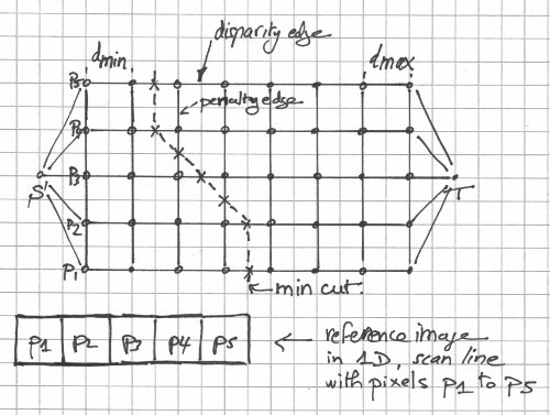
The "graph cuts" method illustrated, in one dimension. From "Stereo Matching and Graph Cuts" by Zureiki, Devy, and Chatila.
The disparity edges are given a weight that corresponds to the "data" energy term. The transverse (penalty) edges are given a weight that relates to the "smooth" energy term. A graph cut separates the graph into two parts, one that connects to the source (S) and one that connects to the sink (T). In 2d, it looks like a curve. In 3d, it looks like a surface. Its weight is the sum of the edge weights. The minimum graph cut (graph cut with minimum weight) corresponds to the minimum energy and that's what you want to find. If you think of the edge weights as pipe capacities in a flow network, finding the min-cut is equivalent to finding the maximum flow. The edges that carry their maximum flows (saturated edges) make up the min-cut.

"Graph cuts" is an elegant and clever approach but, unfortunately, not all energies can be minimized and graph construction can be a tad tricky. It's gotta be the most popular stereo matching global method out there (well, in the academic world, at least). For now, of course.

For a more in-depth view of graph cuts as applied to the stereo matching problem, please check Stereo Matching and Graph Cuts and Stereo Matching and Graph Cuts (Part 2) on this very blog.

Simulated Annealing

"Simulated annealing", as the name suggests, simulates the behavior at the atomic level of a metal that has been heated up and cooled down very slowly. The goal of annealing is to get the metal to a minimum energy state, or at least a very low one.

In simulated annealing, you keep perturbing the current energy state (by changing the disparity of a pixel at random, for example), always accepting a new neighbor state if the energy goes down and possibly accepting a new higher energy neighbor state depending on some probability distribution that's temperature dependent (the lower the temperature, the lower the odds of accepting a higher energy state).

"Simulated annealing" is extremely slow. You not only have to let the temperature go down slowly, you also have to keep perturbing the energy states at a given temperature. Speed improvements can be made by choosing the proper generation probability distribution for the neighboring states (see "fast annealing" and "very fast annealing").

Stereo Matching - Local Methods

In stereo matching (correspondence), local methods attempt to match two dimensional windows (blocks) on the left and right images using a winner-take-all approach (best match wins). They vary by how they compute the matching cost (what matching metric is used) and how they aggregate the cost (how far around the pixel of interest they go). They are local not because of the way they compute the cost but because of the way the problem is solved: For each pixel on the left or right image, a matching pixel is found on the "target" image independently of the other pixels. Contrast this with global methods which minimize the energy of the whole system. Local methods are (much) faster than global methods, that's why they are quite popular. The depth maps obtained by using local matching methods typically suffer from a lack of smoothness, and that's where the global methods come in (we'll check those out in another post).

Let's have a look at the most popular matching metrics in no particular order:



Normalized Cross-Correlation (NCC), Sum of Squared Differences (SSD), Sum of Absolute Differences (SAD) matching metrics.

Most stereo matching algorithms do not make use of RGB color information as they only consider the intensity I, that is, the gray scale value (which varies from 0 to 255). In the formulas, I_bar is the mean intensity value and d is the disparity. The summation is over a window which is usually but not necessarily centered on the pixel to match. The formulas assume that the matches are made along a scan line (v).

Matching a pixel from image 1 to image 2 requires the computation of the matching cost with the disparity d varying from its minimum value to its maximum value (usually given). The lowest cost is taken as the winner (winner-takes-all) and a match is made. It's kinda like sliding (pixel by pixel) the window along the scan line in image 2 and picking the best match (lowest matching cost). Maybe a picture might help:



Window-based stereo matching.

The normalization process in Normalized Cross-Correlation (NCC) reduces the effect of intensity variations between the two images by subtracting the mean from the intensity. Dividing by the standard deviations restricts the Normalized Cross-Correlation to the range [-1,1]. The physical meaning of Normalized Cross Correlation may possibly be better understood if it is shown to be the dot product of two normalized vectors of dimension w x h (where w and h define the window width and height, respectively).



Normalized Cross Correlation (NCC) as the dot product of 2 normalized vectors.

There is no ideal window size: must be big enough to have enough intensity variation to ensure proper matching, but small enough to avoid the effects of perspective distortion (how an object looks against a background usually depends on the point of view).

There are other matching metrics but these three (NCC, SSD, and SAD) are the most common. Which one is the best? It kinda depends on who you are talking to, the kind of images you are dealing with, and how fast you want the matches to be made (clearly, NCC is slower than SSD or SAD).

Stereo Matching - Rectified Geometry

In general, in stereo photography, the image planes (image sensors in digital photography) are not necessarily co-planar and aligned with each other, among other things. Rectification remedies this problem with the end result being that a point in space projects to two location on the same scan line (same row, if you will) in the left and right camera images.



Rectified stereo geometry (3d view).

In the diagram above, O_l and O_r are the optical centers (lens centers) for the left and right lenses. Each image plane defines a two-dimensional coordinate system: a pixel in the left image is defined by its coordinates (x_l,y_l) and a pixel on the right image is defined by its coordinates (x_r,y_r). The point P projects to (x_l,y_l) on the left image plane and (x_r,y_r) on the right image plane such that y_l=y_r=y. The line (row) at ordinate y is a scan line.

In reality, the image planes are positioned behind the optical centers (at f, where f is the focal length) but placing them in front makes it easier because you don't have to deal with image inversion.

If you consider the plane (O_l,O_r,P), the image planes are reduced to the scan line:



Rectified stereo geometry (scan line view).

The vertical lines emanating from the optical centers are the optical axes (lens axes) - they are exactly parallel to each other. The disparity for point P is defined as d=x_l-x_r. Once you know the disparity of a point, geometry of the stereo camera (focal length and baseline, the distance between the two optical centers) gives its depth in the scene.

Dense stereo matching (or correspondence) consists in finding the disparity for every pixel in the left and/or right image (depth map). It is a difficult problem for many reasons (we will look into those in turn in future posts). When the stereo images are rectified, the complexity of stereo matching is slightly reduced (the hard part resides elsewhere).