Automatic depth map generation, stereo matching, multi-view stereo, Structure from Motion (SfM), photogrammetry, 2d to 3d conversion, etc. Check the "3D Software" tab for my free 3d software. Turn photos into paintings like impasto oil paintings, cel shaded cartoons, or watercolors. Check the "Painting Software" tab for my image-based painting software. Problems running my software? Send me your input data and I will do it for you.
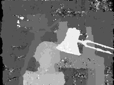
Depth map obtained by DMAG5 using min disparity = -54, max disparity = 25, window radius = 30, alpha = 0.9, truncation (color) = 7, truncation (gradient) = 2, epsilon = 4, and Nbr of smoothing iterations = 0.
This is actually a pretty good depth map with good smoothness except in the lower body area. Of course, the depth for the background is completely wrong but that's an easy fix in post-processing.
Corresponding occlusion map.
The black pixels in the occlusion map indicate areas where the evaluated depth in the depth map is questionable. Black pixels are supposed to show up in occluded areas (areas visible in only one of the two images), in areas where there's no texture, and in areas where the texture is repeated. Black pixels that appear in other areas indicate a problem somewhere. Here, you can see black pixels showing up at the bottom of the image for no real good reason.
Depth map after (minimal) post-processing in Gimp.
Clearly, I've fixed the background depth but I have also worked in the lower part of the image. I've used Gimpel3d to render the 3d scene and The Gimp to modify the depth map. The way I work in The Gimp is by making selections in "quick mask" mode using the left image and painting over the selections in the depth map (When you paint over a selection, you can be pretty sloppy because you cannot change what's not in the selection aka the mask.) I always save my selections as channels just in case they might be needed later.
Wigglegram made with Gimpel3d and The Gimp.
I've used Gimpel3d to generate the frames on either side of the left image and The Gimp to make the animated gif (It's quite easy to do using "Open as Layers" in the "File" menu.) The youtube video below shows the process (for posterity):
DMAG5b is a variant of Depth Map Automatic Generator 5 where the smoothing of the raw cost is performed without preserving the edges of the reference/guide image (it's a simple averaging). This means that DMAG5b is reduced to a winner-takes-all window-based stereo matcher. This type of stereo matching algorithms have a tendency to fatten object boundaries as the window radius increases. They can however be extremely accurate within objects.
Let's go over the parameters that control DMAG5's behavior:
- Minimum disparity is the disparity corresponding to the furthest point in the background.
- Maximum disparity is the disparity corresponding to the closest point in the foreground.
I suggest using Disparity Finder 2 (DF2) to get the minimum and maximum disparity.
- Window radius is the window size. The larger the radius, the more accurate the matches are supposed to be (to a certain extent). If the window radius becomes too large, errors are likely to appear at object boundaries.
- Alpha is the term that balances the color matching cost and the gradient matching cost. The closer alpha is to 0, the more importance is given to the color. The closer alpha is to 1, the more importance is given to the gradient. In theory, a higher alpha works better when there's quite a bit of texture in the image while a lower alpha works better when the image is relatively flat color wise.
- Truncation value (color) limits the value the color matching cost can take. It reduces the effects of occluded pixels (Pixels that appear in only one image.)
- Truncation value (gradient) limits the value the gradient matching cost can take. It reduces the effects of occluded pixels.
In theory, depth map quality is supposed to increase with the thresholds but only to a certain point (If the thresholds are increased too much, quality actually degrades.)
- Disparity tolerance (occlusion detection). The larger the value, the more mismatch is allowed (between left and right depth maps) before declaring that the disparity computed at a pixel is wrong. Obviously, the larger the value, the less black the occlusion map will look.
- Window radius (occlusion smoothing)
- Sigma space (occlusion smoothing)
- Sigma color (occlusion smoothing)
Here's an example:
Depth map obtained by DMAG5b for the Tsukuba stereo pair using a small radius.
Depth map obtained by DMAG5b for the Tsukuba stereo pair using a large radius.
The windows executable (guaranteed to be virus free) is available for free via the 3D Software Page. Please, refer to the 'Help->About' page in the actual program for how to use it.
DMAG5 is very dependent on the so-called "guided filter", which is an approximation of the (joint) bilateral filter. How to compute the guided filter is explained in great details here: Guided Image Filtering.
DMAG5 is similar in spirit to Depth Map Automatic Generator 2 (DMAG2). Just as DMAG2, it is local and filter-based. The difference is that DMAG2 uses a joint bilateral filter while DMAG5 uses a guided filter. The advantage of the guided filter over the joint bilateral filter is that its running time is independent of the filter size (window radius). While DMAG2 is slow (painfully slow if the window radius is not small), DMAG5 is fast. I believe DMAG5 is a real improvement over DMAG2 although one could make the argument that DMAG2 should produce better (more accurate) depth maps than DMAG5 (DMAG5 uses an approximation of the bilateral filter after all). My (limited) experience tells me that DMAG5 produces depth maps that are about as good as those produced by DMAG2.
The cost-volume filtering is performed twice (the first run has the left image as the reference image while the second run has the right image as the reference image) in order to detect occluded pixels. Here, an occluded pixel is a pixel for which the disparity is unreliable. For any found occluded pixel, the disparity is obtained by considering the smallest disparity scanning to its left and to its right. To reduce the streaks in the depth map, occluded pixels are smoothed.
Let's go over the parameters that control DMAG5's behavior:
- Minimum disparity is the disparity corresponding to the furthest point in the background.
- Maximum disparity is the disparity corresponding to the closest point in the foreground.
I suggest using Disparity Finder 2 (DF2) to get the minimum and maximum disparity. Better yet, you can use Epipolar Rectification 9b (ER9b) to rectify/align the two images (crucial for good quality depth map generation) and get the min and max disparities automatically.
- Window radius is the guided filter size. The larger the radius, the more accurate the matches are supposed to be (to a certain extent). If the window radius becomes too large, errors are likely to appear at object boundaries. It is usually a good idea to try radii of various values, like 4, 8, 16, 32, etc. Note that the running time is not dependent on the window radius, which is a really good thing. Please note: The larger the image, the larger the radius should be.
- Alpha is the term that balances the color matching cost and the gradient matching cost. The closer alpha is to 0, the more importance is given to the color. The closer alpha is to 1, the more importance is given to the gradient. In theory, a higher alpha works better when there's quite a bit of texture in the image while a lower alpha works better when the image is relatively flat color wise.
- Truncation value (color) limits the value the color matching cost can take. It reduces the effects of occluded pixels (pixels that appear in only one image).
- Truncation value (gradient) limits the value the gradient matching cost can take. It reduces the effects of occluded pixels (pixels that appear in only one image).
Pauline Tal et al. think that the default truncation values given by Christoph Rhemann et al. (7 for the color truncation and 2 for the gradient truncation) are too small. They suggest 20 and 10 for the color and gradient truncation values, respectively.
- Epsilon controls the smoothness of the depth map. As epsilon is lowered (4, 3, 2, 1, 0, -1, -2, -3, -4, etc), the depth map gets smoother.
- Disparity tolerance (occlusion detection). The larger the value, the more mismatch is allowed (between left and right depth maps) before declaring that the disparity computed at a pixel is unreliable.
- Window radius (occlusion smoothing).
- Sigma space (occlusion smoothing).
- Sigma color (occlusion smoothing).
The parameters that relate to occlusion detection and smoothing should probably be left alone since they only have an effect on the "occluded" pixels, that is, the pixels that show up in black in the occlusion maps.
- Downsampling factor. This parameter enables DMAG5 to run faster by downsampling the images prior to computing the depth maps. If set to 1, the images are used as is and there's no speedup. If set to 2, the images are resized by reducing each dimension by a factor of 2 and DMAG5 should go 4 times faster. The more downsampling is requested, the faster DMAG5 will go, but the more pixelated the depth maps will look upon completion (as they are upsampled). If downsampling is turned on, the parameters that are spatial, that is, min and max disparity, window radius, window radius (occlusion smoothing), and sigma space (occlusion smoothing) are automatically adjusted to adapt to the level of downsampling that is requested. In other words, you don't have to wonder if you should change those parameters when switching, for example, from downsampling factor = 1 to downsampling factor = 2 as DMAG5 does it automatically for you.
The parameters that have the greatest impact on the depth maps are the radius of the guided filter (window radius) and epsilon. So, if you want to experiment, those are the ones you should play with.
The windows executable (guaranteed to be virus free) is available for free via the 3D Software Page. Please, refer to the 'Help->About' page in the actual program for how to use it.
The method described in Weighted Windows for Stereo Correspondence Search (it's called "Adaptive Support-Weight" or ASW in short) created quite a stir in the computer vision community because it was the first time somebody had implemented a local method that was on par with the best global methods. Unfortunately, the problem with ASW (and that's a big one) is that it can be terribly slow especially when the window radius gets large (needed when dealing with larger images). The crux of the ASW method is the use of a filter that's quite similar to the joint bilateral filter, a covolution filter that gives larger weights to the pixels that are similar in color and closer in space to the center pixel (around which the convolution is made). If only there existed a filter similar to the joint bilateral filter that could be implemented so that the running time is independent of the convolution window radius! Well, there is one, it's Guided Image Filtering. Now, how on Earth do you use the guided image filter for stereo correspondence? We'll get to this a bit later.
Usually, in local methods, for each pixel in the left image, one slides a window across the disparity range in the right image and compute some kind of aggregated matching cost at each disparity. When you aggregate the matching costs over a window, you are basically smoothing or filtering the matching costs. A Winner Takes All (WTA) approach is usually employed to get the most appropriate disparity. Another way to do this whole thing is to, for each disparity, compute the raw matching costs at each pixel (no aggregation) and then smooth the raw matching costs that you have just computed. Once you have smoothed all the slices of the cost volume (Each slice corresponds to a disparity.), the same WTA approach can be used to get the most appropriate disparity for each pixel. The advantage of the latter is that you can use any image filter you want to do the smoothing. Since we know that the guided filter can be implemented in such a way that its running time doesn't depend on the window radius, it is a very attractive way of doing local stereo correspondence. This is exactly what Christoph Rhemann et al. did with their fast cost volume filtering. Since the guided filter is quite similar to the joint bilateral filter (used in the adaptive support weights method), we can expect results that are similar and get there fast.
The following describes a bit better the duality between sliding a window across the right image and smoothing the cost volume:
The pseudo-code for the cost-volume filtering shown above is exactly what Christoph Rhemann et al. describe in their paper. Each slice of the cost volume is smoothed by the guided filter which behaves like the joint bilateral filter but is much faster (if the implementation is done right).
This is the raw matching cost Christoph Rhemann et al. use in the paper:
This shows how the weights for the guided filter look like (they look very similar to weights one would get with a bilateral filter):
A couple of disparity maps obtained by the fast cost-volume filtering procedure:
This methodology gets all the accuracy previously obtained by Kuk-Jin Yoon et al. in their adaptive support-weight (ASW) approach and the speed associated with the guided filter. This is, in my opinion, the best local stereo matching algorithm. It also competes quite well with the global stereo correspondence methods like those based on graph cuts.
The guided image filter is a filter that preserves the edges of the guidance image. It behaves quite similarly to the joint bilateral filter but it can be implemented in such a way that its running time is independent of the filter size (the radius of the convolution kernel). Obviously, it can be used for smoothing an image when the guidance image is the input image but it can also be used in stereo matching. The following slides show how to compute the guided image filter when the guidance image is grayscale and color. It is heavily based upon Guided Image Filtering by Kaiming He, Jian Sun, and Xiaoou Tang.
Whenever you need to do a sum over a window, you use the box filter. There is a quite clever implementation of the box filter that makes its running time independent of the window size. This is a very big deal! The method is explained below and it was first presented in "Summed-Area Tables for Texture Mapping" by Franklin C. Crow in 1984.
For convenience, I have compiled all the images in this post into a pdf file: Guided Image Filtering.
DMAG2 generates a depth map by matching windows/blocks in the two images. It's a completely local method. The greater the window radius, the more accurate DMAG2 is. Of course, the larger the window, the slower DMAG2 is, as well. DMAG2 computes two depth maps, one for each image. The two depth maps are checked for consistency and the matches that are not consistent are flagged. The matches that were flagged for inconsistency are shown in black in the occlusion map. At any black pixel, the depth computed with image 1 as the reference image doesn't match the depth computed for image 2 as the reference image. For any of those flagged pixels, the depth is recomputed using adjacency information. The depth maps DMAG2 produces are corrected depth maps.
Truly occluded pixels (present in only one of the two images) will certainly show up in the occlusion map but they aren't the only ones. Pixels in areas of low texture will most likely show up too. To reduce the number of mismatched pixels, it would be a good idea to increase the window radius. To a certain point, of course. I would limit the window radius to a value of 17. If you go past 17 for the window radius, the gamma proximity parameter should be set to the window radius.
Occlusion map (window radius = 12). This shows all the pixels (in black) where the depths are questionable.
Depth map with image 1 (left image) as reference (window radius = 12).
Just for fun, this is what you get if you increase the window radius to 17:
Occlusion map (window radius = 17).
Depth map with image 1 (left image) as reference (window radius = 17).