Stereo Matching - Global Methods

In stereo matching (correspondence), global methods rely on the minimization of an energy functional. This energy functional is usually defined as the combination of a data energy and a smoothness energy.



Example of an energy functional (data and smoothness) to be minimized. From "A Stochastic Approach to Stereo Vision" by Barnard.
The data energy is often borrowed from the local matching methods, as it is often based upon matching metrics like NCC, SSD, or SAD. The smoothness energy is there to penalize disparity solutions that are not smooth (in reality, disparity solutions should really be piecewise smooth). This smoothness energy term is usually derived from the work by Tikhonov on the regularization of ill-posed problems.

Now, what is a bit bothersome about that global energy approach is the fact that two seemingly unrelated energies (data and smoothness) can be somehow combined into one total energy (the "apples and oranges" problem). That's why the smoothness energy is scaled (multiplied) by the regularization parameter (weight) lambda. Now, figuring out what this regularization parameter should be is not exactly easy. You neither want to over-smooth (lambda is too large) nor under-smooth (lambda is too small) the disparity solution. It's usually given a series of values until there's one that seems to give the proper balance between the data energy and the smoothness energy (see L-curves by Hansen for something a little bit more involved).

Given a left and right image of dimension (n x m) and a disparity range (d_min,d_max), you have a total of (d_max-d_min)^(n x m) possible energy states. Finding the minimum energy state by visiting all possible energy states is clearly not feasible (would take exponential time), you therefore need to find a (clever) way to minimize the energy in reasonable time.

Several methods exist to minimize this global energy. In this post, I will only talk about "graph cuts" (GC) and "simulated annealing" (SA).

Graph Cuts

"Graph cuts" solves the minimization problem using graph theory, in particular, the min-cut/max-flow theorem.



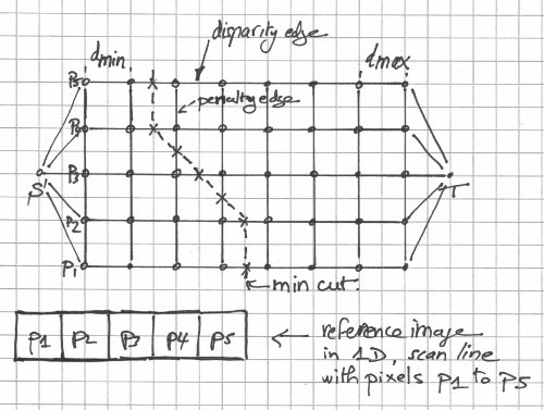
The "graph cuts" method illustrated, in one dimension. From "Stereo Matching and Graph Cuts" by Zureiki, Devy, and Chatila.
The disparity edges are given a weight that corresponds to the "data" energy term. The transverse (penalty) edges are given a weight that relates to the "smooth" energy term. A graph cut separates the graph into two parts, one that connects to the source (S) and one that connects to the sink (T). In 2d, it looks like a curve. In 3d, it looks like a surface. Its weight is the sum of the edge weights. The minimum graph cut (graph cut with minimum weight) corresponds to the minimum energy and that's what you want to find. If you think of the edge weights as pipe capacities in a flow network, finding the min-cut is equivalent to finding the maximum flow. The edges that carry their maximum flows (saturated edges) make up the min-cut.

"Graph cuts" is an elegant and clever approach but, unfortunately, not all energies can be minimized and graph construction can be a tad tricky. It's gotta be the most popular stereo matching global method out there (well, in the academic world, at least). For now, of course.

For a more in-depth view of graph cuts as applied to the stereo matching problem, please check Stereo Matching and Graph Cuts and Stereo Matching and Graph Cuts (Part 2) on this very blog.

Simulated Annealing

"Simulated annealing", as the name suggests, simulates the behavior at the atomic level of a metal that has been heated up and cooled down very slowly. The goal of annealing is to get the metal to a minimum energy state, or at least a very low one.

In simulated annealing, you keep perturbing the current energy state (by changing the disparity of a pixel at random, for example), always accepting a new neighbor state if the energy goes down and possibly accepting a new higher energy neighbor state depending on some probability distribution that's temperature dependent (the lower the temperature, the lower the odds of accepting a higher energy state).

"Simulated annealing" is extremely slow. You not only have to let the temperature go down slowly, you also have to keep perturbing the energy states at a given temperature. Speed improvements can be made by choosing the proper generation probability distribution for the neighboring states (see "fast annealing" and "very fast annealing").