An example of 2D to 3D conversion using Gimpel3D

Lately, I've been looking into ways to convert 2d flat images into 3d scenes, either directly or via a depth map. One can certainly create depth maps using Photoshop or Gimp but I have always been intrigued by 3d scene reconstruction. One program (free and runs on windows) that can do that has caught my eye: Gimpel3D. Gimpel3D was originally written to convert video streams but it can certainly be used to convert a single frame or image (although it might be a tad overkill just to get a depth map).

The documentation for Gimpel3D is not the best but you can pretty much figure out what all the tools do thanks to the html "help" inside the program. There are some things that are not very well explained though, in particular, the "Alignment Options" and "Gap Fill".

Something that should be stressed: Whatever you do in Gimpel3D in terms of modeling, when you look straight on at the scene from the virtual camera (the red dot when Views->Show Camera is checked), you will always see the 2d picture you loaded as if the scene were flat. This explains why things may look weird when you look at the 3d scene from different view points.

In the following youtube video, I've tried to reconstruct the Mona Lisa (actually, a close-up) using Gimpel3D:


Here's the corresponding depth map:

As you can see, there are some problems: the nose is a bit on the manly side and the eye sockets are set way too deep. There's also a depth discontinuity between the face and the hair on both sides. It's not really Gimpel3D's fault as the model file for the human head is probably not the greatest for our Mona Lisa.

Here's another youtube video where I attempt to model the nose of the Mona Lisa using 5 planes (layers) and the "orientation" tool:


Here's the depth map:

I guess I could have also used the "scale" tool but kinda forgot about it when I made the video. In theory, one could model the whole face manually using a bunch of facial planes (see books about drawing the human head). That would certainly be a bit tedious, especially knowing that there's the capability to project onto models. If you don't have a model file handy for an object in the foreground you want to render precisely, I am afraid that there might not be much of a choice. One could also probably use the "contour extrusion" tool and the "anchor points" tool to speed up the "dimensionalization" of an object. I've tried those and they work quite well (as described), but obviously these tools have their own limitations.

3D Photos - Art

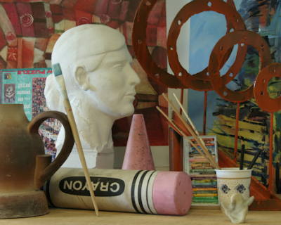
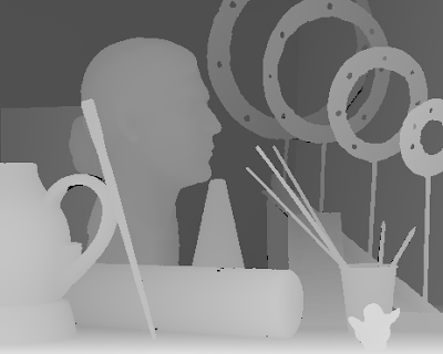
In this post, we are gonna have a look at the stereo pair called "Art" from the Middlebury 2005 Stereo datasets with ground truth and see if we can get a reasonable depth map with Depth Map Automatic Generator (DMAG3) using various lambda values.

Here's "Art" with its ground truth:

Left image

Right image

Ground truth (supplied by Middlebury)

This is not an easy stereo pair to deal with because of the occlusions. Let's give DMAG3 a shot using different values for lambda:

Depth map obtained with DMAG3 (lambda=0)

Occlusion map obtained with DMAG3 (lambda=0)

Depth map obtained with DMAG3 (lambda=1)

Occlusion map obtained with DMAG3 (lambda=1)

Depth map obtained with DMAG3 (lambda=10)

Occlusion map obtained with DMAG3 (lambda=10)

3D Photos - Dolls

Let's consider the stereo pair "Dolls" from the Middlebury 2005 Stereo datasets with ground truth:

Left image

Right image

Ground truth (that's the depth map we rally want to get automatically)

We're gonna use Depth Map Automatic Generator 3 (DMAG3) to generate a depth map using various values for the parameter lambda:

Depth map (lambda=0)

Occlusion map (lambda=0)

Depth map (lambda=10)

Occlusion map (lambda=10)

Depth map (lambda=20)

Occlusion map (lambda=20)

The larger lambda is, the smoother the depth map looks, as expected. At some point, however, the object boundaries are bound to become blurred and accuracy becomes an issue. It should be noted that "Dolls" is an easy stereo pair to deal with since you have a lot of non-repeating textures.

Frame Sequence Generator 3 (FSG3)

Frame Sequence Generator 3 (FSG3) generates synthesized frames given a left image (image 1), a disparity/depth map, and the min and max disparities (needed to compute the actual disparity from the depth map). The basic idea is, for each frame, to shift the pixels in the left image according to the disparity map. This shifted image contains "holes" (areas made up of pixels that have become disoccluded or disoccluded areas, in short) which need to be inpainted (inpainting is a common theme in computer vision. It's pretty easy to understand why you have "holes" showing up when you shift a reference image according to a disparity/depth map. Consider a picture with an object in the foreground with disparity 0 and a background. When you shift the background, "holes" will form on the immediate right of the foreground object. FSG4 fills the "holes" by propagating the pixels to the immediate right of the disoccluded areas using a methodology similar to Semi-Automatic 2D to 3D Image Conversion using Random Walks. This type of inpainting is quite a bit fancier than what's being done in Frame Sequence Generator 2 (FSG2) and therefore, FSG3 should be used in lieu of FSG2.

If imageL.xxx is the left image (image 1), the frames generated will be named frame1.xxx, frame2.xxx, etc. The last frame corresponds to the right image. Animated gifs or lenticular prints (see Lenticular Printing - Interlacing with SuperFlip) can be made with imageL.xxx, frame1.xxx, frame2.xxx, etc (don't use the actual right image). The program automatically creates an animated gif of those images after generating and saving the frames.

The disparity/depth map should be a grayscale image where white indicates closest foreground object and black indicates furthest background object. The darkest value in the depthmap corresponds to the minimum disparity and the brightest value corresponds to the maximum disparity. The disparity/depth map doesn't need to come from any of my programs.

The quality of the inpainting heavily depends on the accuracy of the depth map at object boundaries.

Here's an example:

Left image of the "Art" stereo pair (courtesy of Middlebury).

Depth/disparity map.

Disoccluded areas ("holes") which result from the shifting of the reference image (left image) to get the "right" image (generate 1 frame).

Right image obtained with FSG3.

The windows executable (guaranteed to be virus free) is available for free via the 3D Software Page. Please, refer to the 'Help->About' page in the actual program for how to use it.

Depth Map Automatic Generator 3 (DMAG3)

DMAG3 is an automatic depth/disparity map generator based on the Graph Cuts methodology. It is an implementation of the algorithm described in "Computing Visual Correspondence with Occlusions using Graph Cuts" by Vladimir Kolmogorov and Rabin Zabih. Please refer to Stereo Matching and Graph Cuts and Stereo Matching and Graph Cuts (Part 2) for details about the implementation of such an algorithm, which, by the way, would have not been possible without the help of "Kolmogorov and Zabih's Graph Cuts Stereo Matching Algorithm" by Vladimir Kolmogorov, Pascal Monasse, and Pauline Tan and the accompanying code. I didn't code the actual mincut/maxflow solver. It comes straight from Vladimir Kolmogorov's software library (big thanks to him for providing that).

I recommend having a look at Depth Map Generation using Graph Cuts to get a better grasp of what DMAG3 does and, if nothing else, the meaning of the parameters that control DMAG3's behavior.

The input to DMAG3 is a pair of rectified images as well as the minimum and maximum disparities. The minimum and maximum disparities can be obtained manually with DF2 or automatically with ER9b. I always recommend using ER9b because it rectifies the images but you can also use Stereo PhotoMaker to align the images (although it won't be as good). The output of DMAG3 is the left and right depth maps as well as the left and right occlusion maps.

I think the only parameters to worry about are K and lambda. K is the occlusion penalty. Lambda is the multiplier for the smoothness penalty. For starters, I recommend letting DMAG3 compute K and lambda by setting them both to 0. These 2 parameters should then be modified (if needed) based upon how the left depth map and left occlusion map look. If the occlusion maps look a bit too busy (occluded pixels should only show up at object boundaries), increase K. If the depth maps looks a bit too noisy, increase lambda. If the images are large, I recommend using ds_factor (downsampling factor) = 2 (or more) in order to speed up DMAG3 (tremendously).

Here is an example:

Rectified left image of stereo pair called IMAG0013.

Left depth map obtained by DMAG3.

Left occlusion map obtained by DMAG3.

Here's another example:

Rectified left image of stereo pair called IMAG0020.

Left depth map obtained by DMAG3.

Left occlusion map obtained by DMAG3.

The windows executable (guaranteed to be virus free) is available for free via the 3D Software Page. Please, refer to the 'Help->About' page in the actual program for how to use it.

Weighted Windows for Stereo Correspondence Search

We have previously looked into local methods to solve the stereo correspondence problem using windows (blocks) but we have kind of assumed that the contribution of a pixel around a reference pixel always carry the same weight, in other words, any pixel in the window contributes the same whether it's near or far from the reference pixel and/or its intensity is similar to or different from the reference pixel. This is something we are gonna delve into next thanks to "Adaptive Support-Weight Approach for Correspondence Search" by Kuk-Jin Yoon and In So Kweon. This is akin to adaptive-window methods but handled in a much simpler and natural way.

The idea is to give pixels in a window centered on a reference pixel a weight that depends on spatial proximity and color similarity. This allows the use of a fixed window size unlike the usual adaptive-window methods. You can find the very same methodology in bilateral filtering which is commonly used as an edge preserving blurring/smoothing tool in image processing.

Given a reference pixel p and a neighboring pixel q, this is how the support weight w(p,q) is computed:

Clearly, support weights will vary between 0 and 1. A weight is closer to the value 1 (maximum weight) if its color is similar to that of the reference pixel and it is near the reference pixel. A weight is closer to the value 0 (minimum weight) if its color is not similar to that of the reference pixel and/or it is far from the reference pixel.

Let's look at how the weight distribution looks like in real-life examples (those are from the paper):

As you can see, the brighter pixels are the pixels which are similar in color to the reference pixel (marked by a rectangle). As you move away from the reference pixel, pixels that are similar in color get darker. Recall that brighter pixels have the heaviest weight and contribute the most to the matching cost. It's like adapting the window contour to the object the reference pixel is a part of. As the color similarity parameter (gamma_c) increases, the bright part of the window gets larger, in other words, more of the window carries a significant weight. It's a bit like increasing the window size in the usual non weight-based methods.

Given a pixel p and a disparity d, the matching cost for a given window size is given by:

This matching cost based on weighted correlation windows can be used in local methods (Winner Takes All approach) but also in global methods (as the data term).

As an update to this little write-up (updated 01/14/2014), I would like to go a bit deeper into the color similarity parameter gamma_c and the proximity parameter gamma_p. When looking at the neighborhood of a given pixel in the context of stereo matching, it is kind of assumed that the neighboring pixels should all be at the same depth, in other words, the pixels within a window/block should all be at the same depth. Obviously, we don't know that beforehand since that's we are trying to determine (the depth). So, it is often assumed that neighboring pixels with different colors are likely to be at different depths. It is clearly not always the case (neighboring pixels with different colors could be at the same depth and neighboring pixels with similar colors could be at different depths). It is however not a bad assumption to make when you want to avoid the possible fattening effect ("foreground-fattening") at boundaries between neighboring zones at different depths, a pretty common occurrence in stereo matching algorithms. So, if you look into a neighborhood or window, you want to see weights that are high (close to 1) when the neighboring pixel is similar in color to the center pixel and weights that are low (close to 0) when the neighboring pixel is not similar in color to the center pixel. This is controlled by the color similarity parameter gamma_c. What you also want is a reduction of the weight as you go away from the center pixel. This is controlled by the proximity parameter gamma_p.

Let's look at the following neighborhood window/block (the reference pixel is at the center), play around with gamma_c and gamma_p, and see what kind of effects it has on the pixel weights:

Let's first focus on the color similarity parameter gamma_c. If you set gamma_p to some very large value, it has no effect on the weights (the weights solely come from the color similarity term.) In the following series of pictures, I am only changing gamma_c and see the effect it has on the weights (black means weight equals 0, white means weight equals 1.) What you wanna see is white where there is red and various shades of gray anywhere else (the further away the color is from red, the blacker it should be):

radius=12, gamma_p=1,000,000, gamma_c=200

radius=12, gamma_p=1,000,000, gamma_c=100

radius=12, gamma_p=1,000,000, gamma_c=50

radius=12, gamma_p=1,000,000, gamma_c=20

radius=12, gamma_p=1,000,000, gamma_c=5

Let's now focus on the proximity parameter gamma_p. If you set gamma_c to some very large value, it has no effect on the weights (the weights come solely from the proximity term.) In the following series of pictures, I am only changing gamma_p and see the effect it has on the weights (black means weight equals 0, white means weight equals 1.) What you wanna see is white at the reference pixel and darker shades of gray as you move away from the center:

radius=12, gamma_c=1,000,000, gamma_p=200

radius=12, gamma_c=1,000,000, gamma_p=100

radius=12, gamma_c=1,000,000, gamma_p=50

radius=12, gamma_c=1,000,000, gamma_p=20

radius=12, gamma_c=1,000,000, gamma_p=5

It is worth noting that if both gamma_c and gamma_p are set to large values, all weights are equal to 1 and the method is basically a classic window-based or block-based stereo matching method.

This last picture shows what happens when you combine the color similarity and proximity effects (color similarity weights multiplied by the proximity weights):

radius=12, gamma_c=100, gamma_p=20

Stereo Matching and Graph Cuts (Part 2)

This is a follow-up to Stereo Matching and Graph Cuts.

We are gonna look at how to build the (proper) graph to solve the problem of stereo correspondence with occlusions. This is basically an explanation of the graph construction process in the source code that accompanies "Kolmogorov and Zabih's Graph Cuts Stereo Matching Algorithm" by Vladimir Kolmogorov, Pascal Monasse, and Pauline Tan. That code is a clever implementation of "Computing Visual Correspondence with Occlusions using Graph Cuts" by Vladimir Kolmogorov and Rabin Zabih. This is probably the best Graph Cuts stereo matching algorithm out there in terms of graph construction because it handles occlusions directly. As a reminder, occlusion maps are usually obtained by generating left and right disparity maps and performing a left-right consistency check between the disparities. Here, the occlusion map is obtained with the disparity map without doing a left-right consistency check. The paper that accompanies the code is great in its own right but the binary variable setup is completely different from what is actually in the code. I don't think it's a bad idea to go through the code and (try to) explain what's going on.

In the code, if p is a pixel in the left image with disparity d, the matching pixel in the right image is p+d. Here, I use a different convention for the disparity, so the matching pixel in the right image is p-d. Basically, I use a different sign for the disparity. It really doesn't make any difference whatsoever.

Let's first look at the energy that needs to be minimized (this corresponds to Match::ComputeEnergy() in the code):

The data_occlusion_penalty function looks something like this:

data_occlusion_penalty(p,d)= 0 if d is occluded
data_occlusion_penalty(p,d)= data_penalty(p,d)-K otherwise

where data_penalty(p,d) can be any data penalty energy function (=0 when p and p-d are considered exact matches in terms of intensity). Now, you might think it would probably make more sense to define the data_occlusion_penalty function as:

data_occlusion_penalty(p,d)= K if d is occluded
data_occlusion_penalty(p,d)= data_penalty(p,d) otherwise

but no, that wouldn't work unless you force var0=1 and varA=1 to be incompatible, which is not something you wanna do (trust me, I tried).

The smoothness_penalty function looks something like this:

The smoothness penalty is higher when the intensities are close to each other, which makes a lot of sense since one would expect two neighboring pixels of similar intensities to have the same disparities.

Now that we have clearly defined our energy to be minimized by Graph Cuts, we need to define the graph nodes (the binary variables) and construct the graph so that, whatever the states of the binary variables (0 or 1), the energy of the cuts in the graph is always equal to the energy computed with ComputeEnergy(). This is referred to as a sanity check in the code, for good reasons. We are gonna minimize the energy using the alpha expansion method which considers a switch to the disparity alpha, where alpha can be any possible disparity between the minimum and maximum disparities.

In the following, the function add_constant(E) adds the energy E to the graph. It doesn't depend on any binary variable. The function add_term1(var,E0,E1) adds the energy E0 if var=0, E1 if var=1. It depends on one binary variable (var). The function add_term2(varA,varB,E00,E01,E10,E11) adds the energy E00 if varA=0 and varB=0, E01 if varA=0 and varB=1, E10 if varA=1 and varB=0, E11 if varA=1 and varB=1. It depends on two binary variables (varA and varB).

We are gonna use two graph nodes per pixel:

Node (binary variable) var0 with var0=0 when the pixel p keeps its disparity d and var0=1 if the pixel becomes occluded (d=occluded)
Node (binary variable) varA with varA=0 when the pixel p keeps its disparity d and varA=1 if the pixel changes its disparity to alpha

The binary variable var0 can be active or inactive, present or non-present. Var0 is active when d is already alpha, inactive otherwise. Var0 is present if d is not occluded, non-present otherwise.
The binary variable varA can be active or inactive, present or non-present. VarA is active when d is already alpha, inactive otherwise. VarA is present if p-alpha is in bounds, non-present otherwise.

Let's build the graph nodes and take care of adding data_occlusion_penalty(p,d) (this corresponds to Match::build_nodes() in the code):

This is done for each pixel p. It's pretty clear we can't allow the pixel p to have a disparity d and a disparity alpha, therefore we need to prevent the case (var0=0,varA=1) from ever happening. This is enforced in Match::build_uniqueness_LR():

Now, the fun part is to make sure that whatever the state of the graph node variables (0 or 1), the graph energy always matches the energy computed with ComputeEnergy(). This is what we are looking at here for the most general case (other cases should be looked at in a similar fashion for good measure):

We can clearly see that the energy obtained with build_nodes() matches the energy that we would obtain with ComputeEnergy(), which is a really good thing.

Let's take care of the smoothness terms (this corresponds to Match::build_smoothness() in the code):

This is done for each pixel p and its neighboring pixel np. What's going on regarding the smoothness terms smoothness_penalty(p,np,d) and smoothness_penalty(p,np,nd) is not that clear, to say the least. Here's the explanation for smoothness_penalty(p,np,d):

Here's the explanation for smoothness_penalty(p,np,nd):

We need to force some things in order for the occlusions to show up properly. You don't want to allow a situation where you have, at the same time, a pixel p with disparity d (with matching pixel p-d in the right image) and another pixel p' switching to disparity alpha where p'-alpha happens to be equal to p-d. Indeed, the two pixels would end up having the same matching pixel in the right image, which violates the matching uniqueness. The uniqueness of matches is being enforced in Match::build_uniqueness_RL() in the code and it's reproduced here:

This is done for each pixel in the right image. Note that the code always keeps track of disparities in the right image as expansion moves are performed (if pixel p in the left image has disparity d, pixel p-d in the right image has disparity -d.)

That's about it, really. Now, if you think that having two sets of binary variables seems unnecessary and that having just one set of binary variables and letting expansion moves go to the occluded state would work just about the same, well, you'd be wrong (I know, I've tried). What would happen is that even though you would reach a lower energy state, a good number of pixels would be given a disparity even though they should really be occluded. The key to proper occlusion detection is enforcing the right to left uniqueness, and this can only be done with two sets of variables (I think.)